Some notes on sampling from character-level RBMs
This is a (somewhat boring and technical) accompaniment to my blog post Dreaming of GitHub repositories with RBMs. I was able to find lots of great literature with practical tips on training RBMs (my favourite being Geoff Hinton’s A Practical Guide to Training Restricted Boltzmann Machines), but almost nothing on sampling from them. This may reflect the fact that generative models have more often been used to pretrain discriminative models rather than, y’know, generate stuff.
My hope is that these notes might help out any future ML archaeologists who want to hack around with RBMs. The TL;DR is:
simulated annealing is one honking great idea – let’s do more of that!
Background - Gibbs sampling
(If you’re already familiar with RBMs, feel free to skip this part.)
One of the fundamental operations we can perform on an RBM is called Gibbs sampling.
    def gibbs_sample(self, visible):
        hidden = self.sample_hidden(visible)
        return self.sample_visible(hidden)

    def sample_hidden(self, visible):
        """Sample from P(h|v)"""
        hidden_probs = logistic(np.dot(visible, self.W.T) + self.visible_bias)
        return np.random.rand(hidden_probs.shape) < hidden_probs

    def sample_visible(self, hidden):
        """Sample from P(v|h)"""
        visible_probs = logistic(np.dot(hidden, self.W.T) + self.hidden_bias)
        return np.random.rand(visible_probs.shape) < visible_probs
Gibbs sampling starts from some configuration of one of the layers, and essentially bounces back and forth between the visible and hidden layers, continually asking “What hidden states go well with these visible states?”, then “What visible states go well with these hidden states?”.
Here’s an example of how the state of the visible layer evolves during repeated Gibbs sampling. This example uses a model trained on a dataset of geographical place names:
| i | visible | energy(visible) |
|---|---|---|
| 1 | tyxeavonam adhbufwij | 35.4 |
| 2 | tenrimilty in dlenic | -19.2 |
| 3 | gedromoold in foerna | -21.0 |
| 4 | eo wiogh in fulrsa | -21.7 |
| 5 | cl biigs in fusrta | -24.2 |
| 6 | lhgwiogs in filrma | -20.8 |
| 7 | sogwiitt on fueeso | -29.2 |
| 8 | mockiotd on lueera | -34.9 |
| 9 | commaosy an luvera | -30.1 |
| 10 | seroont on lemert | -35.8 |
| 11 | g an sun lerort | -42.8 |
| 12 | toon yan ferert | -55.6 |
| 13 | doin ron forest | -61.0 |
It’s not a coincidence that the energy is going down over time, or that the sample with the lowest energy is the one that looks most like a real name. There’s a connection between how we do sampling and our energy function above. The probability of turning on a particular hidden unit h_j, given a visible vector v is:
1 / 1 + exp(-1 * (hidden_bias[j] + W[j]*v))
If the model doesn’t care about h_j and gives it a bias of 0, and all its weights 0, then the exponent goes to 0, and the probability of turning on becomes 1/2. As we decrease the bias, or give it negative weights at indices where v is turned on, then the energy associated with that unit being on increases, and the probability goes toward 0. If we do the opposite, the effect on energy becomes negative, and the probability goes to 1. So, the probability of turning on a hidden unit is proportional to the negative energy difference associated with turning it on. The same argument applies to visible units conditioned on hidden vectors.
Remember how RBMs are trying to learn the distribution of our data? An important property of RBMs is that if we do Gibbs sampling over and over, our samples will approach the model’s estimation of that distribution.
Softmax sampling
One thing to notice for character-level RBMs in particular is that, for every block of N visible units representing a character, there will always be exactly one unit turned on - the probability we assign to any vector failing this criterion should be 0. We should help the network out by giving it this information for free. We’ll do that by treating each of those blocks as a single ‘softmax’ unit. Rather than sampling each visible binary unit independently, and turning it on with some probability according to the sum of the incoming weights from the hidden layer, we’ll sample using the softmax function.
This isn’t strictly necessary, but I found it to greatly improve the model (in terms of qualitative goodness of samples, and some metrics that correlated well with quality of samples, such as pseudolikelihood).
Drawing samples
Once we’ve trained a model, we want to see what kinds of hilarious garbage it dreams up. How do we do that? Well, we know that if we start anywhere and do Gibbs sampling long enough, we’ll get something like the model distribution. There’s even a proof of it in a drawer somewhere! Problem solved, right?
In practice, “long enough” might be a long, long time for some models. An RBM (or, more generally, any Markov chain) that takes a long time to converge is said to have a low mixing rate. Such models may wallow in valleys of (locally) low energy for a long time, and be very sensitive to initial conditions.
Here’s (ugly HTML table warning) what a well-behaved model looks like. Each row represents a different starting point for the sampling, and each line is a separate “fantasy particle”, sampled in parallel (if you’re curious about the meaning of each row, check out the VisInit enum here). The samples in the final column of each row (representing 10k iterations of sampling) are fairly similar, and there’s no evidence of any particles getting stuck. After 10k iterations, the training examples are substantially transformed.
Here’s what a bad mixing rate looks like. Even after 10k iterations, there are dramatic differences in samples depending on how the chains were started. chunks/silhouettes/train look pretty reasonable, but the chains started from zeroed-out vectors look like noise. Many of the chains started from training examples still look a lot like their starting configuration - e.g. “carleton pond dam” -> “greslocd ponn dam”, “southwestern college” -> “southordoure college”).
One way to avoid the second scenario is to introduce a weight cost to discourage large weights, which are associated with poor mixing rates.
Journey to Goon Remetery
Let’s consider a sample from our well-behaved model: “goon remetery”. Ouch, so close. But remember that our procedure for sampling the visible units is stochastic. It may be that we had P(“r”) = 0.1, P(“c”)=0.8 for index 5, and that we just got unlucky. To maximize the quality of our samples, we could sample determnistically at the very last round of sampling, always taking the character with the highest probability.
This is actually how I drew samples initially, until a friend pointed out to me that this is actually a (trivial) special case of simulated annealing. To take it further, we’ll need to introduce the concept of “temperature” to the sampling process:
    def sample_hidden(self, visible, temperature):
        """Sample from P(h|v)"""
        hidden_probs = logistic(np.dot(visible, self.W.T/temperature) + self.visible_bias/temperature)
        return np.random.rand(hidden_probs.shape) < hidden_probs
When temperature=1.0, we have our normal sampling procedure. Other temperature values will scale our weights and biases up or down. A high temperature has the effect of flattening out the probability distribution. In the limit, when T is infinite, we’ll ignore the weights and biases, setting the hidden units with a coin flip (and setting the visible units with the flip of a ~26-sided coin).
A low temperature has the effect of “sharpening” the probability distribution, with the rich getting richer and the poor getting poorer. T=0 leads to exactly the procedure we described earlier where we always take the character with the highest score.
Simulated Annealing
We can draw our samples with simulated annealing by starting our chain at a high temperature and gradually lowering it. This is appealing for a few reasons:
Firstly, it defeats models with low mixing rates. Recall that our problem was fantasy particles stubbornly lying in local valleys. Turning up the heat will bounce them out and encourage them to explore other regions.
It also lets us draw samples with much lower energy than what we would get from repeated Gibbs sampling at T=1 - even after many iterations. And low energy samples tend to be qualitatively superior. We can no longer pretend that we’re trying to draw from exactly the model distribution - we may be drawing from a sharpened version of that distribution that favours especially probable points. In practice, we’re totally cool with this, as long as we still get some reasonable variety.
Examples
Here are some samples drawn after 1000 rounds of Gibbs sampling on a model trained on GitHub repository names:
  cyilagct-buarcs
  DCG-arrales
  mbd_ppp_scrip
  Coursers-NHSI_SIC
  OrilinguCoFLR
  jeadio_rubs
  My-tant4.jl
  GetNeI
  Kcsoolstorjs-Domo
  jx-nitkmesu
Yikes!
Here are samples from the same model, with the same number of iterations, but annealing from T=1.5 to T=0.2:
 cloud-pron-pyshin
 learns_sample_app
 simple-checking
 vinital-config
 openbone-backer
 grunt-test
 CSCI-2014
 testRepose
 iO-LibyAnalysis
 Java-Android-Test
Wow! Quite the difference.
Where did 1.5 and 0.2 come from? Annealing schedules are kind of black magic here. I tried a lot of them, and different models liked different schedules. Here’s one example of average energy over time for a bunch of different annealing schedules:
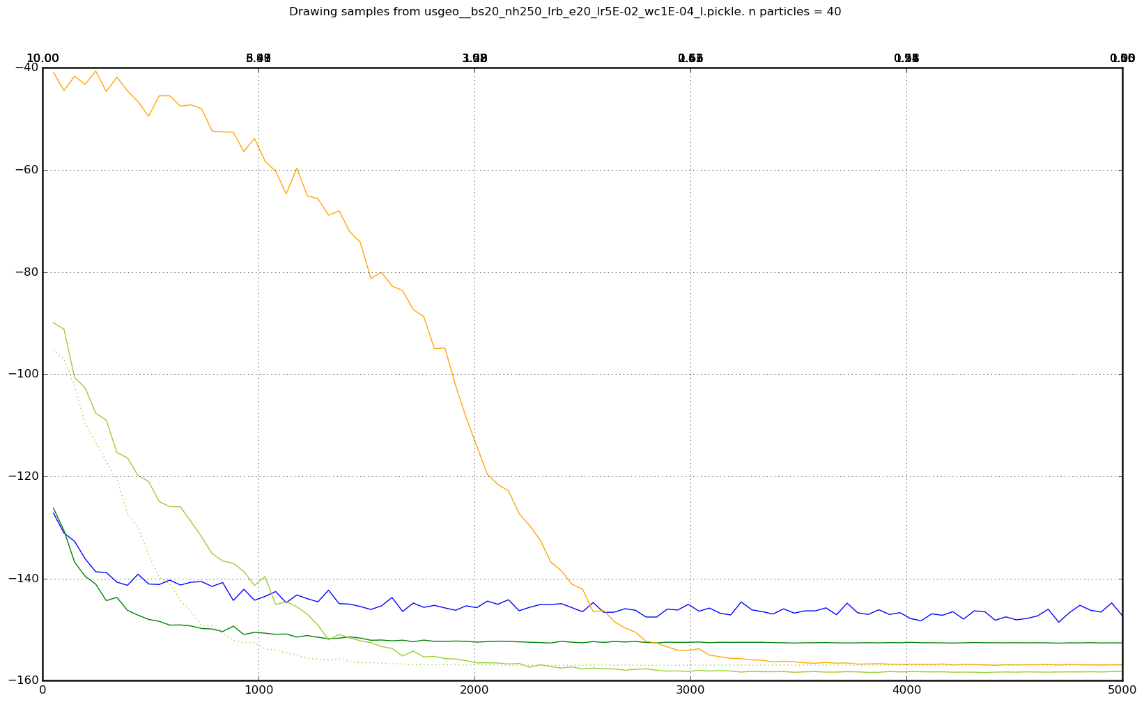
Apologies for the messiness. It probably would have been a good idea to label the lines, because I definitely can’t remember the temperatures associated with each of those lines (but higher y-intercept -> higher starting temperature, steeper slope -> lower ending temperature). The important thing here is that the blue line is with no annealing. So pretty much any reasonable annealing schedule trounces vanilla Gibbs sampling, if your goal is to get lower energy samples.
But getting low energy samples is probably not all you care about. Often a gentle annealing schedule will give the lowest average energy, but lead to very low sample diversity. For example, here are some samples taken over a gentle annealing period from a model trained on names:
aaron           lee
mark            lee
jan             man
jess            lee
adam            lee
al              man
jason           lee
henry           lee
leo             mana
jason           mane
At this point, we’ve probably sharpened the distribution too much. We probably want to cool a bit faster to before every particle has had a chance to fall into the valley of the Lees.
For reasons like this, I relied pretty much entirely on visual inspection of samples when choosing annealing schedules.
Tagged: Machine Learning