Dissecting Google's Billion Word Language Model Part 1: Character Embeddings
Earlier this year, some researchers from Google Brain published a paper called Exploring the Limits of Language Modeling, in which they described a language model that improved perplexity on the One Billion Word Benchmark by a staggering margin (down from about 50 to 30). Last week, they released that model.
As someone with an interest in character-aware language models, I’ve been looking forward to sniffing around this thing.
In this post, I’ll go into the very first layer of the model: character embeddings.
Background - language models
To begin with, let’s define what we mean by a language model. A language model is just a probability distribution over sequences of words. Given a sentence like “Hello world”, or “Buffalo buffalo Buffalo buffalo buffalo buffalo Buffalo buffalo”, the model outputs a probability, telling us how likely that sentence is.
Language models are evaluated by their perplexity on heldout data, which is essentially a measure of how likely the model thinks that heldout data is. Lower is better.
The lm_1b language model takes one word of a sentence at a time, and produces a probability distribution over the next word in the sequence. Therefore it can calculate the probability of a sentence like “Hello world.” as…
P("<S> Hello world . </S>") = product(P("<S>"),  P("Hello" | "<S>"),
    P("world" | "<S> Hello"), P("." | "<S> Hello world"),
    P("</S>" | "<S> Hello world ."))
("<S>" and "</S>" are beginning and end of sentence markers.)
The lm_1b architecture
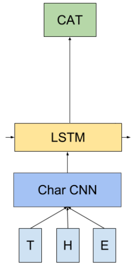
The lm_1b architecture has three major components, shown in the image on the right:
- The ‘Char CNN’ stage (blue) takes the raw characters of the input word and produces a word-embedding.
- The LSTM (yellow) takes that word representation, along with its state vector (i.e. its memory of words it’s seen so far in the current sentence), and outputs a representation of the word that comes next.
- A final softmax layer (green) learns a distribution over all the words of the vocabulary, given the output of the LSTM.
Char CNN?
This is short for character-level convolutional neural network. If you don’t know what that means, forget I said anything - because in this post, I’ll be focusing on what happens before the network does any convolving. Namely, character embeddings.
Character embeddings?
The most obvious way to represent a character as input to our neural network is to use a one-hot encoding. For example, if we were just encoding the lowercase Roman alphabet, we could say…
onehot('a') = [1,0,0,0,0,0,0,0,0,0,0,0,0,0,0,0,0,0,0,0,0,0,0,0,0,0]
onehot('c') = [0,0,1,0,0,0,0,0,0,0,0,0,0,0,0,0,0,0,0,0,0,0,0,0,0,0]
And so on. Instead, we’re going to learn a “dense” representation of each character. If you’ve used word embedding systems like word2vec then this will sound familiar.
The first layer of the Char CNN component of the model is just responsible for translating the raw characters of the input word into these character embeddings, which are passed up to the convolutional filters.
In lm_1b, the character alphabet is of size 256 (non-ascii characters are expanded into multiple bytes, each encoded separately), and the space these characters are embedded into is of dimension 16. For example, ‘a’ is represented by the following vector:
array([ 1.10141766, -0.67602301,  0.69620615,  1.96468627,  0.84881932,
        0.88931531, -1.02173674,  0.72357982, -0.56537604,  0.09024946,
       -1.30529296, -0.76146501, -0.30620322,  0.54770935, -0.74167275,
        1.02123129], dtype=float32)
That’s pretty hard to interpret. Let’s use t-SNE to shrink our character embeddings down to 2 dimensions, to get a sense of where they fall relative to one another. t-SNE will try to arrange our embeddings so that pairs of characters that are close together in the 16-dimensional embedding space are also close together in the 2-d projection.
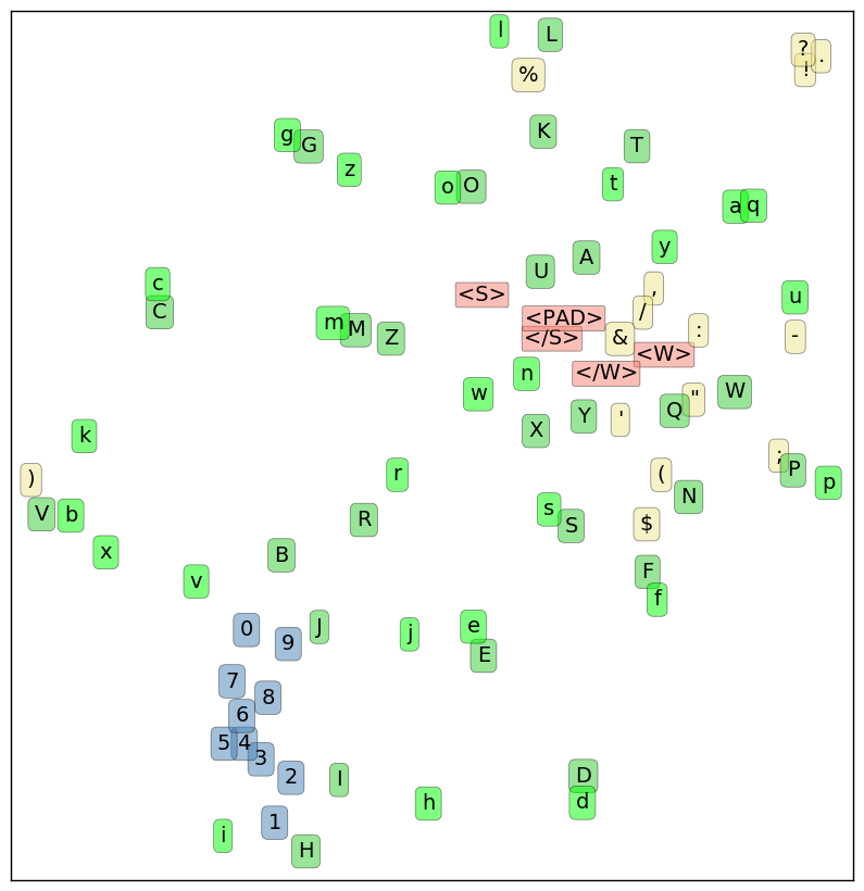
A few interesting regularities jump out here:
- not only are digits clumped closely together, they’re basically arranged in order along a snaky number line!
- in many cases, the uppercase and lowercase versions of a letter are very close. However, a few, such as “k/K” are widely separated. In the original embedding space, 50% of lowercase letters have their uppercase counterpart as their nearest alphabetical neighbor.
- in the upper-right corner, all the ASCII punctuation marks that can end a sentence (
.?!) are in a tight huddle - meta characters (in salmon-pink) form a loose cluster. Non-terminal punctuation forms an even looser one (with “%” and “)” as outliers).
There’s also a lack of regularity that’s worth noting here. Other than the (inconsistent) association of uppercase/lowercase pairs, alphabetical characters seem to be arranged randomly. They’re well-separated from one another, and are smeared all across the projected space. There’s no island of vowels, for example, or liquid consonants. Nor is there a clear overall separation between uppercase and lowercase characters.
It could be that this information is present in the embeddings, but that t-SNE just doesn’t have enough degrees of freedom to preserve those distinctions in a 2-d planar projection. Maybe by inspecting each dimension in turn, we can pick up on some more subtleties in the embeddings?
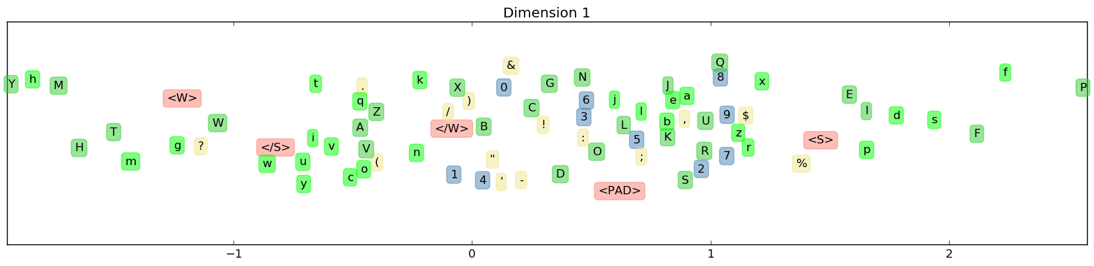
Hm, maybe not. You can check out (bigger) plots of all 16 dimensions here - I haven’t managed to extract much signal from them however.
Vector math
Perhaps the most famous feature of word embeddings is that you can add and subtract them, and (sometimes) get results that are semantically meaningful. For example:
vec('woman') + (vec('king') - vec('man')) ~= vec('queen')
It’d certainly be interesting if we could do the same with character vectors. There aren’t a lot of obvious analogies to be made here, but what about adding or subtracting ‘uppercaseness’?
def analogy(a, b, c):
  """a is to b, as c is to ___,

  Return the three nearest neighbors of c + (b-a) and their distances.
  """
  # ...
‘a’ is to ‘A’ as ‘b’ is to…
>>> analogy('a', 'A', 'b')
b: 4.2
V: 4.2
Y: 5.1
Okay, not a good start. Let’s try some more:
>>> analogy('b', 'B', 'c')
c: 4.2
C: 5.2
+: 5.9

>>> analogy('b', 'B', 'd')
D: 4.2
,: 4.9
d: 5.0

>>> analogy('b', 'B', 'e')
N: 4.7
,: 4.7
e: 5.0
Partial success?
Repeating this a bunch of times, we get the ‘right’ answer every once in a while, but it’s not clear if it’s any better than chance. Remember that half of lowercase letters have their uppercase counterpart as their nearest neighbour. So if we strike off a short distance from a letter in a random direction, we’ll probably land near its counterpart a decent proportion of the time for that reason alone.
Vector math - for real this time
I guess the only thing left to try is…
>>> analogy('1', '2', '2')
2: 2.4
E: 3.6
3: 3.6

>>> analogy('3', '4', '8')
8: 1.8
7: 2.2
6: 2.3

>>> analogy('2', '5', '5')
5: 2.7
6: 4.0
7: 4.0

# It'd be really surprising if this worked...
>>> nearest_neighbors(vec('2') + vec('2') + vec('2'))
2: 6.0
1: 6.9
3: 7.1
Okay, note to self: do not use character embeddings as tip calculator.
It seems useful to embed digits of similar magnitude close to each other, for reasons of substitutability. ‘36 years old’ is pretty much substitutable for ‘37 years old’ (or even ‘26 years old), ‘$800.00’ is more like ‘$900.00’ or ‘$700.00’ than ‘$100.00’. And based on our t-SNE projection, it seems like the model has definitely done this. But that doesn’t mean that it’s arranged the digits on a line.
(For one thing, there are probably some digit-specific quirks the model needs to learn. For example, that years usually start with ‘20’ or ‘19’.)
Making sense of it all
Before guessing at why certain characters were embedded in such-and-such a way, we should probably ask: why are they using character embeddings in the first place?
One reason could be that it reduces the model complexity. The feature detectors in the Char CNN part of the model only need to learn 16 weights for every character they’re looking at, rather than 256. Removing the character embedding layer increases the number of feature detector weights by 16x, from ~460k (4096 filters * max width of 7 * 16-dimensional embedding) to ~7.3m. That sounds like a lot, but the total number of parameters for the whole model (CNN + LSTM + Softmax) is 1.04 billion! So a few extra million shouldn’t be a big deal.
In fact, lm_1b uses char embeddings, because their Char CNN component is modeled after Kim et. al 2015, who used char embeddings. A footnote from that paper gives this explanation:
Given that |C| is usually small, some authors work with onehot representations of characters. However we found that using lower dimensional representations of characters (i.e. d < |C|) performed slightly better.
(Presumably they mean better performance in the sense of perplexity, rather than e.g. training speed.)
Why would character embeddings improve performance? Well, why do word embeddings improve performance in natural language problems? They improve generalization. There are a lot of words out there, and a lot of them occur infrequently. If we tend to see “raspberry”, “strawberry”, and “gooseberry” in similar contexts, we’ll give them nearby vectors. Now if we’ve seen the phrases “strawberry jam” and “raspberry jam” a few times, we can guess that “gooseberry jam” is a reasonably probable phrase, even if we haven’t seen it in our corpus once.
Generalizing over characters?
At first, the analogy with word vectors doesn’t seem like a good fit. The billion word benchmark corpus has 800,000 distinct words, whereas we’re dealing with a mere 256 characters. Is generalization really a concern? And how do we generalize from a “g” to other characters?
The answer seems to be that we don’t really. We can sometimes generalize between uppercase and lowercase versions of the same character, but other than that, alphabetical characters have distinct identities, and they’re going to occur so frequently that generalization isn’t a concern.
But are there characters that occur infrequently enough that generalization is important? Let’s see…
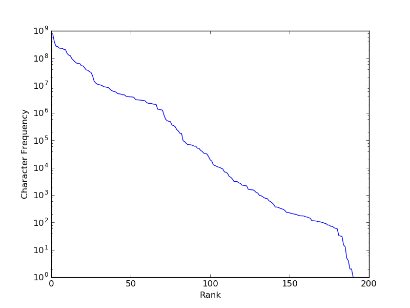
Well, it’s not quite Zipfian (we get closer to a straight line with only the y-axis being on a log scale, as above, rather than with a log-log scale), but there’s clearly a long tail of infrequent characters (mostly non-ASCII code points, and some rarely occurring punctuation).
Maybe our embeddings are helping us generalize our reasoning about those characters. In the t-SNE plot above, I only showed characters that occur fairly frequently (I set the threshold at the least frequent alphanumeric character, ‘X’). What if we plot the embeddings for all characters that appear in the corpus at least 50 times?
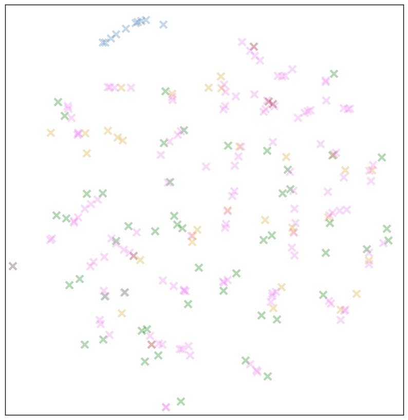
This would seem to support our hypothesis! As before, our letters (green markers), are pretty antisocial, and rarely in touching range of one another. But in several places, our long-tail pink characters form tight clusters or lines.
My (handwavey) best guess: alphabetical characters get distinct, widely-separated embeddings, but characters that occur infrequently (the pinks) and/or characters with a high degree of substitutability (digits, terminal punctuation), will tend to be placed together.
That’s it for now. Thanks to the Google Brain team for releasing the lm_1b model. If you want to do your own experiments on it, be sure to check out their instructions here. I’ve made the scripts I used to generate the visualizations in this post available here - feel free to re-use/modify them, though they’re messy as hell.
Tune in next time, when we’ll look at the next stage of the Char CNN pipeline - convolutional filters!
Tagged: Machine Learning, Data Visualization