A classic problem in natural language processing is named entity recognition. Given a text, we have to identify the proper nouns. But what about the generative mirror image of this problem - i.e. named entity generation? What if we ask a model to dream up new names of people, places and things?
I wrote some code to do this using restricted Boltzmann machines, a nifty (if passé) variety of generative neural network. It turns out they come up with some funny stuff! For example, if we train an RBM on GitHub repository names, it can come up with new ones like…
fuzzyTools
Slick-Android-App
sublime-app
Backbone-Switcher
MODEL1302110000
If you want to flip through more examples, there’s a (web) app for that. Check out…
If you want to learn about how I got there, read on. In this post, I’ll give a brief overview of restricted Boltzmann machines and how I applied them to this problem, and try to give some intuition about what’s going on in the brain of one of these models.
My code is available here on GitHub. Feel free to play with it (with the caveat that it’s more of a research notebook than a polished library).
Restricted Boltzmann Machines
Background - generative models
Our goal is to build a model that spits out funny names, but our path there will be a bit indirect. The problem that RBMs - and generative models in general - are trying to solve is learning a probability distribution. We want to learn a function P that assigns every string a probability according to its plausibility as a particular kind of name. e.g. in the case of human names, we probably want…
P("John Smith") > P("Dweezil Zappa") >> P("mCN xGl JeY")
If we can sample from this distribution, the effect should be like thumbing through a phone book. We’ll see lots of “John Smith”s, we might eventually see a “Dweezil Zappa”, but we’ll probably never find a “mCN xGL JeY”.
Representing Inputs
We’ve said we want to learn a function over strings, but anything we’re going to feed into a neural network needs to be transformed into a vector of numbers first. How should we do that in this case?
Most NLP models stop at the word level, representing texts by counts of words (or by word embeddings, such as those produced by word2vec). But breaking up GitHub repository names (like tool_dbg, burgvan.github.io, or refcounting) into words isn’t trivial. And more to the point, we don’t want to limit ourselves to regurgitating words we’ve seen in the training data. We want to generate whole new words (like, say, Brinesville). For that, we need to go deeper, down to the character level.
We’ll represent names as sequences of one-hot vectors of length N, where N is the size of our alphabet.
Because we’re not using a recurrent architecture, we’ll need to fix some maximum string length M ahead of time. Names shorter than M will need to be padded with some special character.
For example, let’s take our alphabet to be just {a,b,c,d,e,$}, where ‘$’ is our padding character, and set M to 4. We can encode the name ‘deb’ using the following 4x6 matrix:
| index | a | b | c | d | e | $ |
|---|---|---|---|---|---|---|
| 0 | 0 | 0 | 0 | 1 | 0 | 0 |
| 1 | 0 | 0 | 0 | 0 | 1 | 0 |
| 2 | 0 | 1 | 0 | 0 | 0 | 0 |
| 3 | 0 | 0 | 0 | 0 | 0 | 1 |
RBMs
A restricted Boltzmann machine (henceforth RBM) is a neural network consisting of two layers of binary units, one visible and one hidden. The visible units represent examples of the data distribution we’re interested in - in this case, names.

Again, RBMs try to learn a probability distribution from the data they’re given. They do this by learning to assign relatively low energy to samples from the data distribution. That energy will be proportional to the (negative log) learned probability.
In the diagram above, the energy of the RBM will be equal to the negative sum of:
- the biases on the two active (red) hidden units
- the biases on the active (blue) visible units
- the weights connecting the red and blue units (i.e. the bold lines)
There are weights connecting every visible unit to every hidden unit, but no intra-layer (visible-visible, or hidden-hidden) weights. During training, the RBM will adjust these weights, and a vector of biases for the visible and hidden units, in such a way as to bring down the energy of training examples, without bringing down the energy of everything else along with it.
v is defined as sum(energy(v, hidden) for hidden in all_possible_hidden_vectors). We can't feasibly iterate over all 2n possible hidden layers, but it turns out there's an equivalent closed-form that's easy to calculate.
Drawing samples
Once we’ve trained a model, how do we get it to talk? Starting from any random string, we sample the hidden layer. Then using that hidden layer, we sample the visible layer, getting a new string. If we repeat this process (called Gibbs sampling) a whole bunch of times, we should get a name out at the end.
What does it mean to sample the hidden/visible layer? Our binary units are stochastic, so given a string, each hidden unit will want to turn on with some probability, according to its bias and the weights coming into it from active visible units. Sampling the hidden layer given a visible layer means turning each hidden unit on or off according to some rolls of the dice. (And vice-versa for sampling the visible layer.)
More details (for nerds)
If you’re interested in reading more about RBMs, I highly recommend Geoff Hinton’s A Practical Guide to Training Restricted Boltzmann Machines, which was my bible during this project.
I trained my models using persistent contrastive divergence. I used softmax sampling (described in 13.1 of “Practical Guide”) for the visible layer - without it, results were very poor.
Sampling was not quite as simple as my handwaving in the section above would suggest. I used simulated annealing, which turned out to help a lot. I wrote a separate little post about sampling here.
This README has details on hyperparameters used to train each of my models and the annealing schedule used to sample from them.
Results
Let’s look at what some RBMs dreamed up on a few different name-like datasets. This README describes where each dataset was downloaded from and how it was preprocessed.
Any names that existed in the training data were filtered out of the lists below (and in the name generator apps). This cut anywhere between .01% of samples to 10% depending on the model.
Human names
Here are some samples drawn from a model trained on the full names of 1.5m actors from IMDB (more here):
omar vole
r.j. pen
ronald w. males
jean-paul recan
marxel sode
samuel j. varga
lionel cone
(It turns out they meant “actors” in the gendered sense of the word, which is why you won’t see any female names.)
The dataset includes naming traditions from around the world which created several distinct modes that the model captured pretty well. For example, it generates names like…
hiroshi tajamara
hing-hying li
vladimir tjomanovic
giuseppe rariali
But is unlikely to generate a name like “hiroshi tjomanovic”.
(Incidentally, Google tells me that none of “Tajamara”, “Hing-hying”, “Tjomanovic” and “Rariali” are actual extant names - though based on my limited exposure to Japanese/Chinese/Slavic/Italian names, I could have believed they were all real. We want to generate novel examples not copied from the training set, so this is good news.)
The model’s favourite name (that is, the sample it assigned the lowest energy) was christian scheller (who exists in the training set - christian schuller, who doesn’t exist, is a close second).
Geographic names
It’s not much of a stretch of the imagination to go from training on names of people to names of places (examples from the dataset: “Gall Creek”, “Grovertown”, “Aneta”, “Goodyear Heights”). Here are some random examples from our RBM’s dreamed atlas (more here):
sama
marchestee hill
wano
fleminger river
arring lake south
jicky park
mount ono
oste
lake day
Not bad! Who wouldn’t enjoy a picnic in Jicky Park?
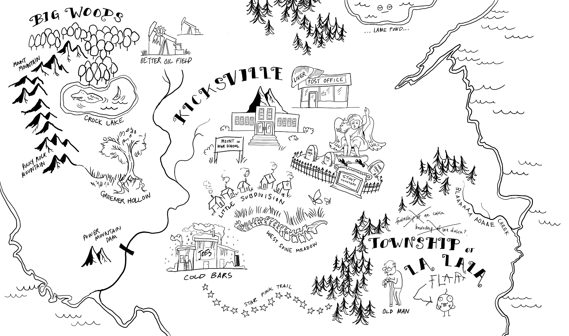
The map at the top of this post is a terrifying vision of a whole territory dreamed up by an RBM - full version here.
The model’s favourite place name was indian post office, which exists in the training set. It’s second favourite is wester post office, which doesn’t.
GitHub repository names
How about some GitHub repos? More here:
frost2
gruntus.js
simpleshefe
backbook.com
thetesters
mandolind
smart-cheling
ShreeCheck
redget-2014
tumber_server
Some of the favourites I jotted down as I hacked on different models:
supervaluation
JustQuery
hello-bool
dataserverclient
bachbone.github.io
2048-ing-master
jonky-howler
PinglePlungerDemo
faceboogler
Model’s favourite name: unity.github.io, which doesn’t exist in the training set.
Bonus: Board games
I spent a bit of time trying to learn board game names, but wasn’t particularly successful. I suspect my dataset, at about 50k games, was just too small. Some samples (more here):
stopeest game
chef ths gome
the mitean game
eleppitt care game
chipling gome
the sidal game
elepes on the game
the hing board game
Well, it’s certainly figured out that the word “game” is important to unlocking the mystery of this distribution. Good job on that, RBM. It caught a few other types of game names, but again with a lot of jpeg compression:
hocket'& pace
spop the gime
brauk
pocket quizs
Favourite name: the : the card game. The most commonly sampled name was the bile game, which appeared 700 times in 35k samples. Neither game exists in the training set. If you do own a copy of The Bile Game, don’t invite me over for board game night.
“Did they really need a neural network for that?”
This is a question that probably doesn’t get asked often enough. The results here are pretty neat, but before we claim another victory for trendy neural networks, we should ask whether the problem we solved was actually difficult. I’ll follow the example of this blog post by Yoav Goldberg and use unsmoothed maximum-likelihood character level language models as a dumb baseline to compare against. In short, we’ll generate strings one letter at a time, choosing the next letter by looking at the last n, and seeing which letters tended to follow that sequence in the training set.
Some examples from an order-4 model trained on the US place names dataset:
Bonny Maringer City of Lake
Sour Motoruk Mountain
Mount Branchorage Lakes
Duck Kill Bar Rock
Goatyard Point
Noblit Hollow
Spenceton
Jay Canal Cemetery
Oriflamming Beach
Huh. Those are, uh, actually pretty excellent. And with 4-grams it’s not at the point where it’s just copying the training data. Around 25% of generated names exist in the training set, but I filtered those out of the list above. Several of the individual tokens above don’t exist in the training set either, including the excellent “Goatyard”.
Let’s see if we can salvage our dignity by comparing performance on the GitHub dataset. The order-4 output is pretty goofy, so let’s give it 5 characters of context:
littlePython-hall-effectv-frontAngles2
media
EasyCanvas
shutupmrnotific
MinkGhost-deployShpaste_ember
terrain-Exercise3
gaben
bot-repots-interestingGithub.io
CredStatus
wall-as
BB-FlappyBao
py_shopping-sample
Our baseline’s not looking so hot now. It’s interesting to note some mistakes here that the RBM model almost never makes. For example, it never flubs the formatting of a URL. It’s also very good at picking a consistent scheme for case and separators for each name, e.g.:
SAPAPP
rails_work_app
DataTownSample
java-mails-rails
This is where being able to see the whole string at once really comes in handy. When our Markov model has generated as far as “java-mails”, it doesn’t have enough context to know whether it should make java-mails-rails or java-mailsRails or java-mails_Rails. We can always feed it even more context, but a window of 5 already leads to a lot of copy-pasting from the training set. For example, shutupmrnotific is funny, but it’s just a truncation of a repo from the training set, shutupmrnotification.
More stupid RBM tricks
The coolest thing we can do with our trained models is ask them to come up with new names, but that’s not the only thing we can ask of them. We can also give them a name of our own choosing and ask them how good they think it is. Let’s see if the model we trained on actor names has the hoped-for behaviour on the example names we described at the beginning:
>>> E('john smith')
-75.10
>>> E('dweezil zappa')
-38.14
>>> E('mcn zgl jey')
-34.25
Remember that lower energy corresponds to higher probability, so this is great! Energy is proportional to the log of the probability, so the model thinks that Dweezil is about 4 orders of magnitude more likely than Mcn, and 37(!) orders of magnitude less likely than John. (That sounds like a lot, but Dweezil is a pretty extreme example of a rare name - it’s globally unique!)
It can be interesting to walk around the neighbours of a name to get a feel for the energy landscape of the model, and its robustness to small changes:

john smith. Names are arranged into columns according to the affected index in the string. Note that the y-axis is reversed.
The chart above is heartening. First of all, it’s great that our model assigned lower energy to the ‘real’ name than to any of the corrupted versions. But the order assigned to the corrupted names also seems very reasonable. The ones with the lowest energy - Messrs. Smitt, Smitz, and Smich - are the most plausible. The three samples with the highest energy are not only weird - they’re not even pronouncable in English.
This is a nice intuitive way of evaluating our model's density function - it seems obvious that our model should generally assign more energy to a sample from our dataset after we've randomly nudged it. It also plays around a key weakness of RBMs: we can't calculate the exact probability they assign to any instance, because of an intractable term called the partition function. But we can compare probabilities. When we take the energy difference between two instances, the partition function cancels out, and we get the exact log-ratio of their probabilities.
In fact, this is the basis for a clever training technique called score matching, which turns out to have a surprising connection with denoising autoencoders, another powerful variety of generative neural network.
Understanding what’s going on
A common trick when working with neural nets in the image domain is to visualize what a neuron in the first hidden layer is “seeing” by treating the weights between that neuron and each input pixel as pixel intensities.

We can do something similar here. The tables below each represent the ‘receptive fields’ of individual hidden units. The columns correspond to positions in a 17-character GitHub repo name. A green character represents a strongly positive weight (i.e. this hidden unit “wants” to see that character at the position). Red characters have strongly negative weights.
These are just a couple examples taken from a model with 350 hidden units (the same model from which the above samples were taken). This page has visualizations of all those units, as well as examples of strings having high affinity for each unit.
| v | n | d | u | b | n | r | L | z | m | . | 6 | v | ||||
| a | a | g | r | l | i | o | _ | k | ||||||||
| r | r | s | m | i | a | e | 4 | |||||||||
| j | R | D | i | a | l | d | 1 | |||||||||
| V | e | b | o | o | t | - | ||||||||||
| E | y | e | e | n | d | y | n | a | G | H | I | E | V | P | P | i |
| o | d | a | o | r | s | - | a | . | . | G | v | J | H | 2 | n | S |
| I | l | q | a | m | c | s | e | $ | - | _ | x | f | w | C | g | a |
| e | s | i | g | t | t | g | i | _ | _ | - | J | y | P | W | - | y |
| i | i | t | t | e | e | n | o | - | $ | . | . | G | _ | . | S | 1 |
This hidden unit wants to see… vndubnr? Actually, this word search is hiding several useful words.
- vagrant
- android
- arduino
- angular
- ansible
This kind of multitasking is a common theme. And maybe it shouldn’t be surprising. This model only has 350 hidden units, but a good model of repository names needs to remember more words than that (not to mention formatting and the phonotactic rules for inventing new words).
Of course, this hidden unit alone is perfectly happy to see hybrid prefixes like vadroid, or andulant or even aaDmaae. It needs to work in concert with other hidden units that impose their own regularities, like…
| B | Y | W | A | n | e | y | Y | |||||||||
| A | _ | V | E | t | o | |||||||||||
| 3 | I | K | a | d | a | |||||||||||
| C | I | b | i | |||||||||||||
| R | o | k | u | |||||||||||||
| s | f | 8 | q | i | 5 | h | ||||||||||
| m | 2 | a | T | e | l | z | ||||||||||
| W | i | Q | C | o | x | 4 | ||||||||||
| x | m | O | r | u | r | c | $ | |||||||||
| w | h | q | l | a | 0 | b | k | 7 |
Whereas the last unit was focused on a few domain-specific words, this unit is pretty generic. It mostly just wants to see a vowel in the fourth position followed immediately by a consonant (note that the chars it least wants to see there are [a, u, o, e, i]). With this and the previous unit turned on, we’re now happy to see ‘angular’ and ‘ansible’, but not ‘vagrant’, ‘android’, or ‘arduino’.
Of course, our model has no explicit knowledge of what a “vowel” is, so it’s neat to see it picked up naturally as a useful feature.
Another emergent behaviour is the strong spatial locality. With few exceptions, hidden units have their strong weights tightly clustered on a particular neighbourhood of character positions. This is neat because, again, we never told our model that certain visible units are “next to” each other - it knows nothing about the input geometry.
A few more examples below.
Making it better
Going Deeper
RBMs can be stacked on one another to form a deep belief network. It seems plausible that additional layers would be able to learn higher layers of abstraction and generate even better samples.
Remember how we saw above that most units learn patterns local to a particular region of the string? This may explain solecisms like Lake Lake, or Church Swamp. If, as seems to be the case, our initial layer of hidden units is mostly learning words, phonotactics, and low-level structural patterns (word lengths, spacing), another layer of hidden units on top of those could learn more semantic patterns. e.g. “Lake $foo”, “$foo Lake”, “$foo Swamp”, but never “Lake Lake”, “Lake Swamp”, etc. I would be sad to see Days Inn Oil Field go though. That one was pretty good.
Translation Invariance
Under the current architecture, for a model to learn the word “Pond” (a very useful word to learn if you want to generate place names), it needs to memorize a separate version for each position it can appear: ___ Pond, ____ Pond, _____ Pond, etc.
We’d like our model to learn robust, position-invariant patterns and understand that “Hays Pond” and “Darby Pond” are quite similar (even though their vector representations are completely disjoint).
One solution to this problem is to use a recurrent architecture. Another, which is more readily applicable to RBMs, is to use convolutional units. If you’re familiar with the use of CNNs for vision tasks, this will sound familiar.
In a convolutional RBM, each hidden unit will only have connections to a small substring of the input. Weakening our hidden units like this doesn’t sound like much of a win, but because each unit has fewer weights, we can use a lot more of them without slowing down training. Not only that, but each hidden unit will work together with many siblings that share the exact same weights but look at different regions of the string. Together these make up what’s called a “filter”.
As an example, the model might learn a filter that recognizes a consonant followed by a vowel anywhere in the string. Imagine taking the consonant-vowel hidden unit from before, and making 15 copies of it, one copy for a vowel at index 0 and consonant at index 1, another copy for vowel at index 1 and consonant at index 2, etc.
Again, the promise of this is strongly suggested by the weights we see on the hidden units above. Our hidden units are already looking at local regions of the input, and there’s clear evidence that the model is having to learn and store the same pattern multiple times for different positions: the hidden unit zoo lists 20 hidden units that seem to be primarily responsible for recognizing github.io and github.com URLs. Some are even pseudo-convolutional, trying to recognize two shifted versions simultaneously.
With convolutional units, we could help the network do what it’s already doing much more efficiently (in terms of the size of the model, and the amount of information learned per training instance).
Practical Applications
None whatsoever.
Acknowledgements
The Unreasonable Effectiveness of Recurrent Neural Networks by Andrej Karpathy inspired me to play with character-level representations (and was basically the first thing I read that got me excited about deep learning). If you haven’t read it already, go do it now! If you’re curious how these results compare to char-rnn, here are some samples from a char-rnn model trained for around 24 hours on GitHub repos with rnn_size=256, seq_length=20 and all other options set to their defaults.
Thanks to Falsifian for reviewing a draft of this post and teaching me about simulated annealing. Thanks to an anonymous brilliant artist for drawing that Tolkien-esque map of “Kicksville” in the header.
Tagged: Machine Learning